Stellar Spot Modeling
Over the past two days I worked on fitting the simultaneous MOST photometry and CHIRON RV measurements of Epsilon Eridani. This document describes some of the more general code as well as the early results. The full spot modeling code will be made publicly available when the peer-reviewed paper is accepted.
####Importing the Data
After finding out over the weekend that the times we stored in IDL data structures (and published over the last 6 years) were erroneous, I used the exposure meter midpoints from the MySQL database instead:
cmd = "SELECT emmnwob, mnvel, errvel FROM exposuremeter e "
cmd += "INNER JOIN velocities v ON v.observation_id = e.observation_id "
cmd += "INNER JOIN observations o ON o.observation_id = e.observation_id "
cmd += "WHERE object=22049 AND tag='a' AND mnvel IS NOT NULL"

engine = ccdb.connectChironDB()

eerv = pd.read_sql_query(cmd, engine)
And converted the exposure meter midpoints to Julian Dates using
the pandas DatetimeIndex and to_julian_date() methods:
emmnwobjds = pd.DatetimeIndex(eerv.emmnwob)
eerv['emmnwobjd'] = emmnwobjds.to_julian_date()
The next step was to restore the MOST data from file and downsample by taking a
running mean. Downsampling reduced the noise and allowed the photometry to
be combined with the RV data without completely dominating the solution.
Both restoring the data and downsampling were accomplished in
pandas with a little help from the Time method in astropy:
from astropy.time import Time
#restore data
eeph = pd.read_csv('epsEriMost.txt', sep='\s+', skipinitialspace=True)
#create JD astropy Time object for easy conversion to ISO format:
MostJds = Time(eeph.MJD + 2451545., format='jd')
#now store as DatetimeIndex
eeph['ObsDT'] = pd.DatetimeIndex(MostJds.isot)

#next create a one column series of flux values with the observation
#time as the index:
eemr = pd.Series(data = eeph['flux'].values, index=eeph['ObsDT'])
mhc = {'Mean' : np.mean}
downsampledtimes = eemr.resample("480min", how = mhc).index.to_julian_date()
downsampledflux = eemr.resample("480min", how = mhc)
Since the MOST data have reported homoscedastic errors (a rarity in astronomy) this worked out. Otherwise, we’d need to take a weighted mean.
####The Maximum Likelihood Method
We would like to fit the spectroscopic and photometric data simultaneously to get a self-consistent model describing the star. For a first step in doing this, I went with a quick maximum likelihood approach. The log likehood function for the problem is:
`[ \ln{p(v, \phi|t, \sigma, t’, \sigma’, \Theta)} = - \frac{1}{2} \sum_{n}\left[ \frac{(v_{n} - f(t_{n}| \Theta))^{2}}{\sigma_{n}^2} + \ln{(2 \pi \sigma_{n}^{2})}\right]
- \frac{1}{2} \sum_{m}\left[ \frac{(\phi_{m} - f’(t’{m}| \Theta))^{2}}{\sigma{m}^{‘2}} + \ln{(2 \pi \sigma_{m}^{‘2})}\right] ]`
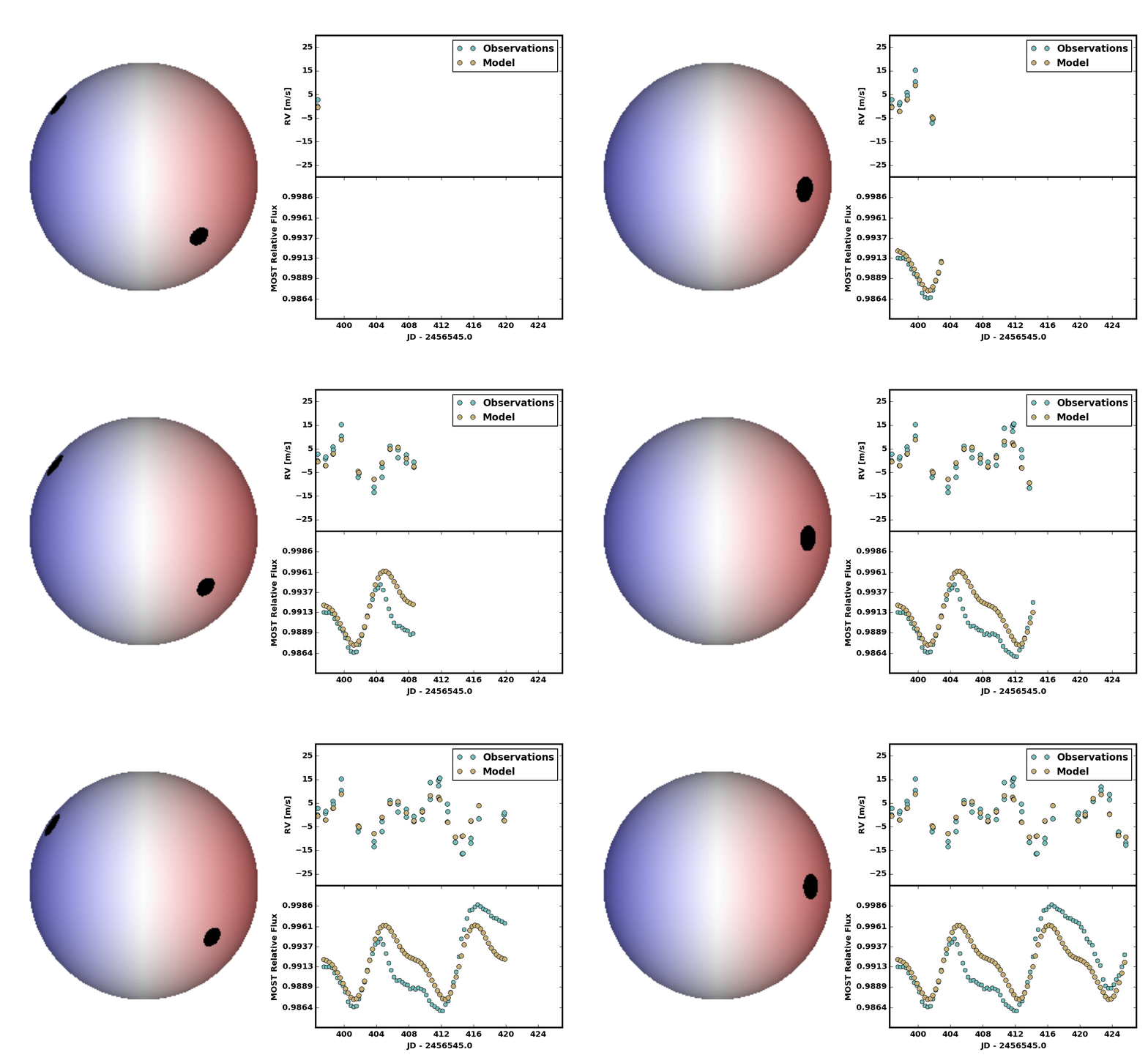
where \(v_{n}\) is the radial velocity measurement for the \(n^{th}\) observation taken at time \(t_{n}\), \(\sigma_{n}\) is the single measurement uncertainty, and \(f\) is the radial velocity spot model given our hyperparamers, \(\Theta\), \(\phi_{m}\) is the flux of the \(m^{th}\) photometric observation happening at time \(t'\), \(f'\) is the photometric spot model given our same hyperparameters, \(\Theta\), and \(\sigma_{m}^{'}\) is the photometric uncertainty of the \(m^{th}\) observation. The hyperparameters here are
- the latitude of spot 1
- the phase of spot 1
- the fractional area of spot 1
- the latitude of spot 2
- the phase of spot 2
- the fractional area of spot 2
This was then driven by minimizing the negative of the log likelihood:
#use the scipy optimize method:
import scipy.optimize as op
nll = lambda *args: -lnlike(*args)
result = op.minimize(nll, theta_init, args=(t, v, verr, t2, f, ferr),
                     method='Powell')
For a first pass we decided to include two spots. No spot growth or decay. No differential rotation. Just something quick and dirty, but it was clear at least two spots were needed. Below is an animation showing the result.
