The CHIRON Barycentric Correction
When using the radial velocity method to search for planets orbiting nearby stars, the dominant signal is always due to the Earth’s motion about the barycenter of the solar system. Our annual orbit induces a signal of 30,000 m/s. Furthermore, as the observatory rotates towards the star, the Earth’s rotation can induce a maximumradial velocity of 400 m/s. If we didn’t correct for these two effects, we would find all sorts of celestial bodies with annual and daily orbits. But to find low mass planets, there are all sorts of other motions and effects that need to be taken into account. For example, if we didn’t account for the presence of Jupiter, we would see a 12 m/s signal with a period of approximately 12 years. For each spectroscopic observation we take, we calculate a precise photon-weighted midpoint of the observation, and then calculate a barycentric correction to subtract from the Doppler measurement. This barycentric correction takes into account the relative motions of all the planets and many minor bodies in the Solar System, the position of the observatory on Earth, leap seconds due to events such as storms and earth quakes on Earth that speed up or slow down the Earth’s rotation, etc. For a great description of all that goes into the barycentric correction, see Barycentric Corrections at 1 cm/s for precise Doppler velocities by Wright & Eastman (2014).
The other day I noticed a rather interesting correlation between the radial velocity measurements and the barycentric correction. It can be seen in the following plot, which shows the RV Measurements as a function of the Barycentric Correction.
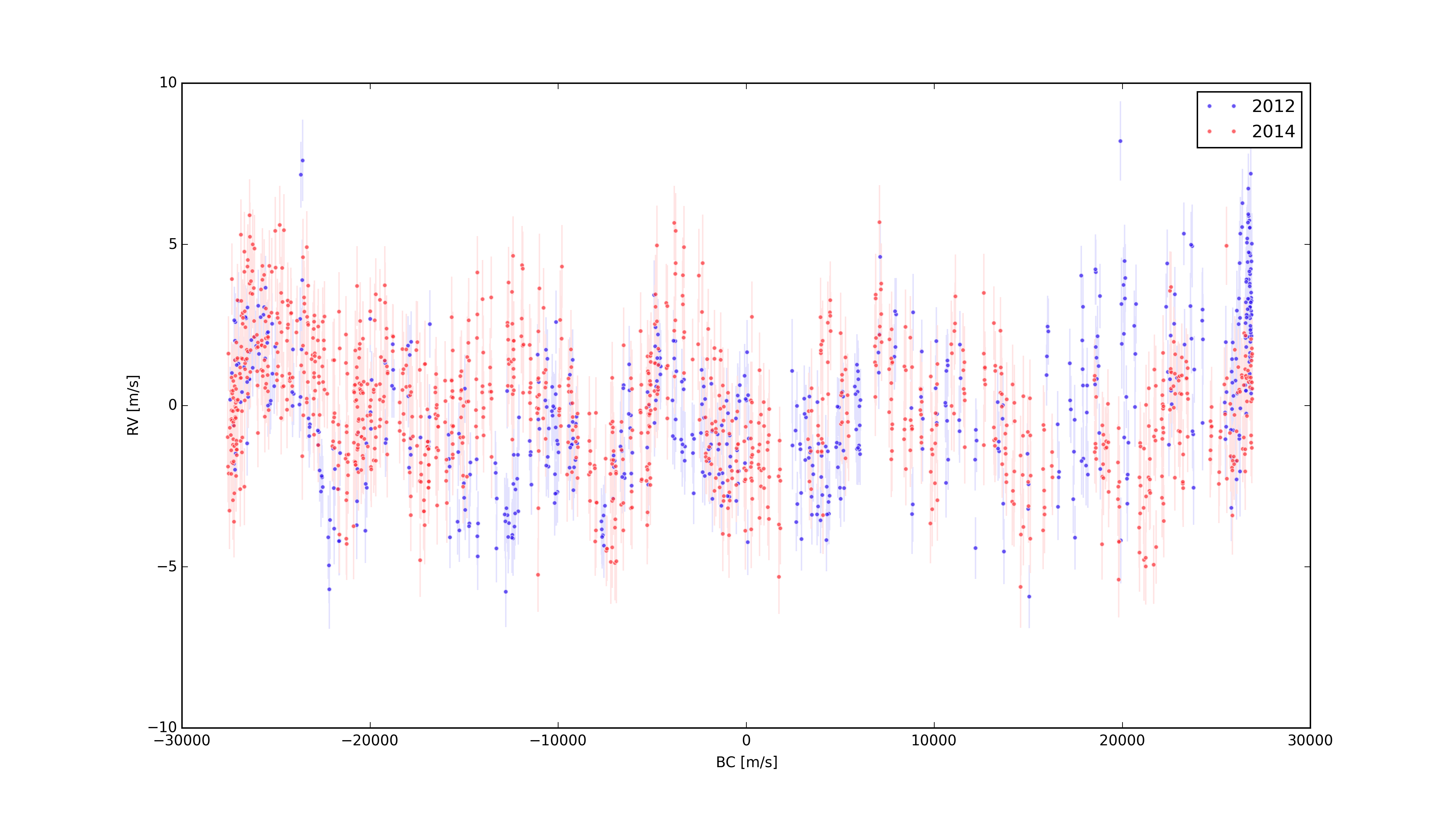
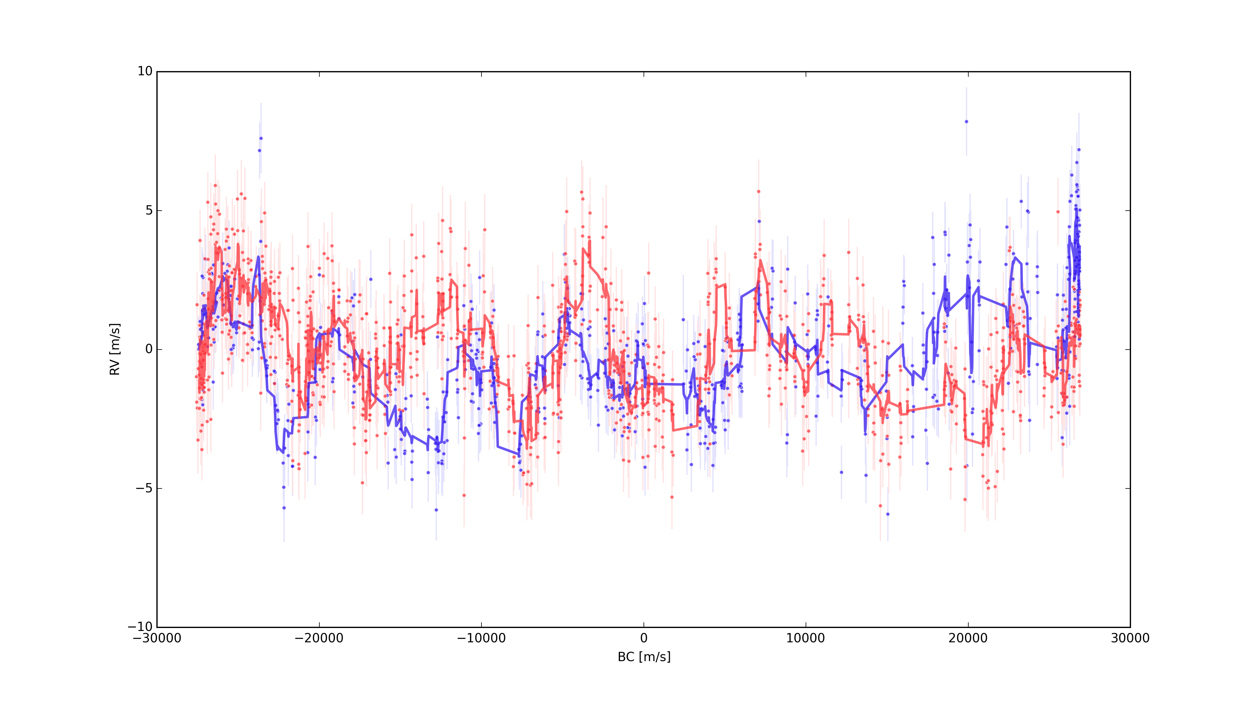
In red are Doppler measurements based on CHIRON observations of Tau Ceti in 2014, and in blue are the same, but based on 2012 data. While the correlation is not perfect, it’s quite clear in a few regions (e.g, < -20,000 m/s, and between -8,000 m/s and 0 m/s). This can be seen a little more clearly by applying a running mean to the data, which can be seen at the solid lines in the following figure.
This signal is not really periodic, so it’s most likely not due to a planet in a perfect harmonic with the Earth’s orbit, and I also wouldn’t expect it to be due to an issue with the barycentric correction for the same reason. However, we want to make sure we have the best barycentric correction possible so that we can find genuine low mass planets and not harmonics of a poor treatment of the motions of celestial bodies in our Solar System. A simple first step was to replace our current barycentric correction code with the improved code by the above mentioned Wright & Eastman (2014). So I downloaded their code, and all the dependencies, setup Launch Daemon scripts to check for daily updates for leap seconds and so forth, and recalculated the barycentric corrections for all of our velocity measurements. The result was an RMS for the Tau Ceti RV time series that was 30 cm/s greater than the RMS from the previous code.
I then started looking into everything that could be wrong. I double-checked that the coordinates I was using were the most accurate. For Tau Ceti this required checking the RA, dec, proper motions, and parallax were all from the Hipparcos New Astrometric Catalog (van Leeuwen (2007)). The whole catalog can be found online on the Vizier site. The data for Tau Ceti in particular can be found here. For CTIO, the most precise coordinates for the 1.5 m were measured by Mamajek (2012). I was indeed already using the most up to date coordinates.
I then decided maybe we can do better than these measurements. We have this great time series of precise RV measurements. Can you we use those measurements to infer a more accurate position of the observatory here on Earth and a more accurate position and relative motions for Tau Ceti? I thought it’d be worth a shot, so I setup emcee on several machines in our group cluster, got MPI running on all the machines, and thought I’d try calculating more accurate hyperparameters through sampling the posterior PDF.
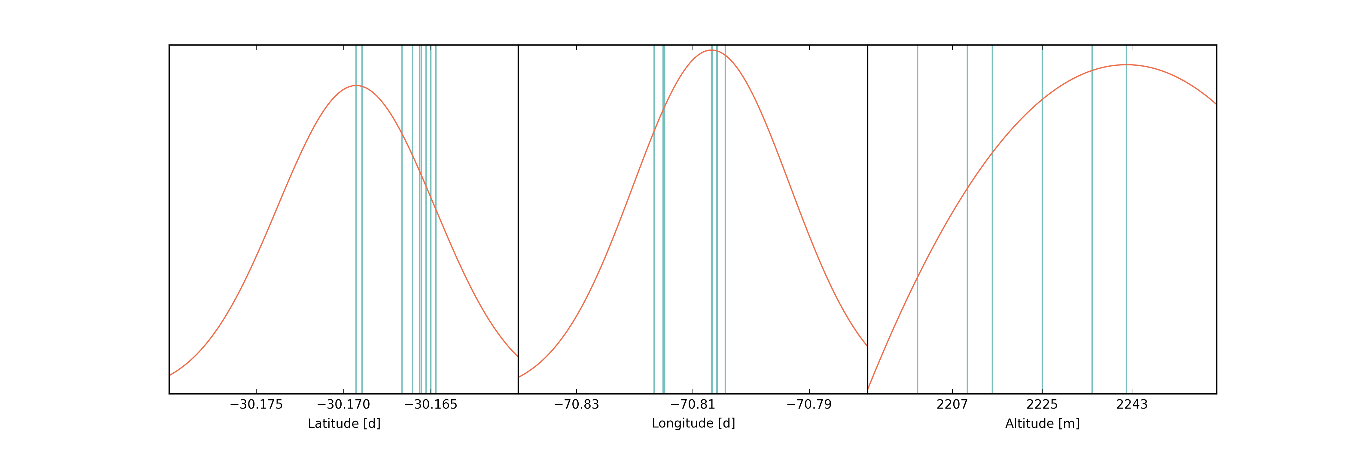
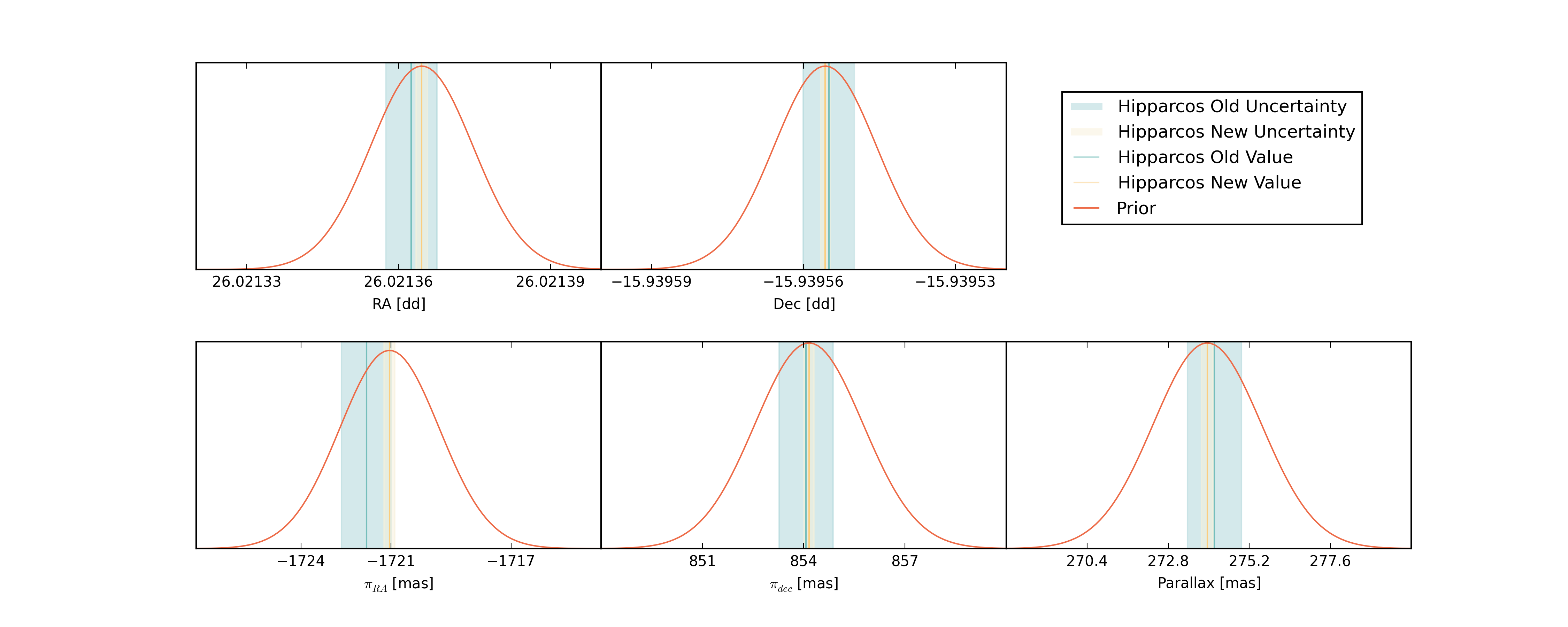
For priors for the observatory position I used Gaussians that were centered on the Mamjek values and had a standard deviations that were a factor of a few larger than the standard deviation of the previously measured values. These priors are shown below, where the vertical blue lines show previously published results, and the red lines show the resulting priors.
For the priors for the coordinates and motions of Tau Ceti I again used Gaussians centered on the Hipparcos data with standard deviations a few times those of their reported uncertainties. These can be seen below, where the values and uncertainties from the intial reduction are shown in blue, and values and uncertainties from the new reduction mentioned above are shown in yellow, and the priors used are shown in red.
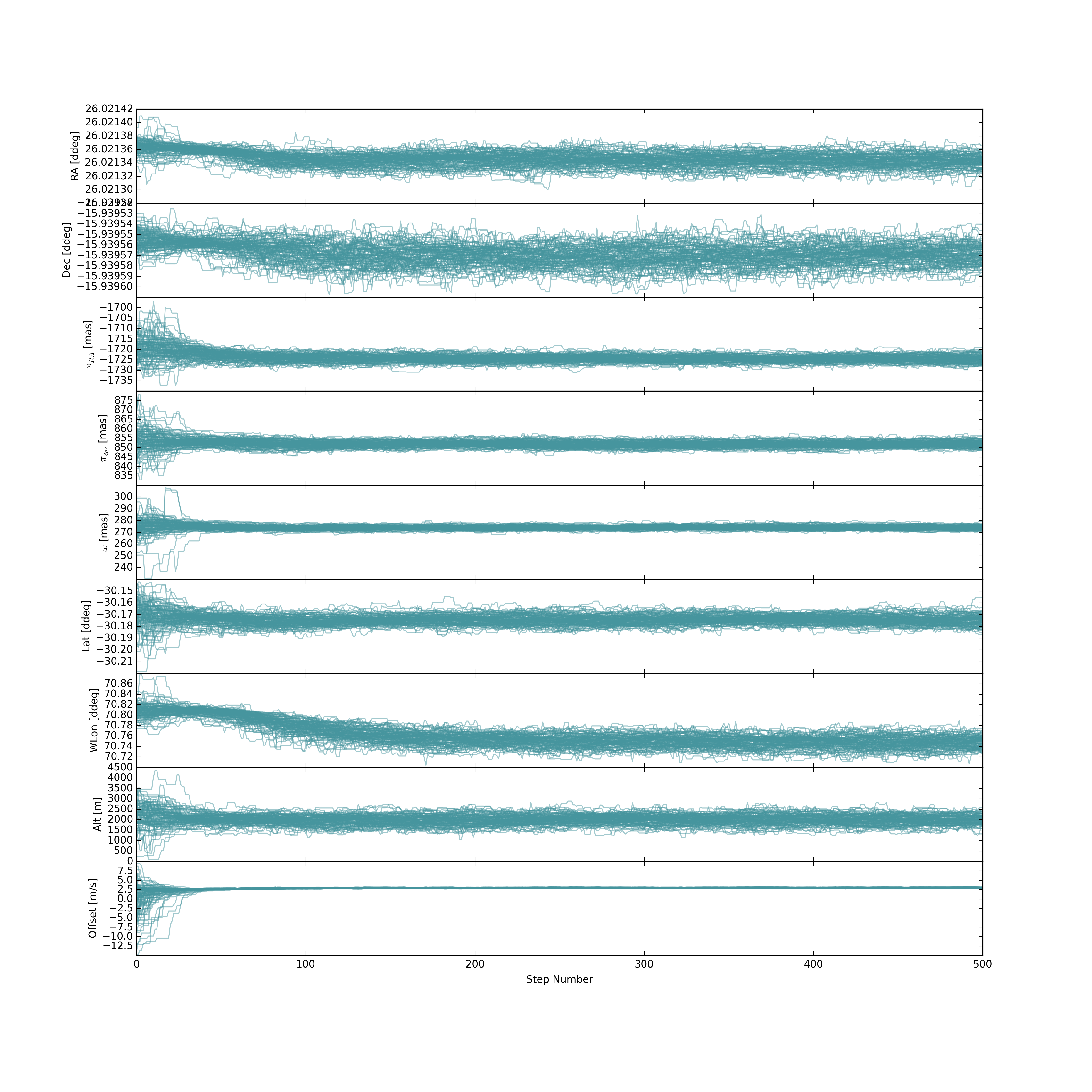
After some tweaking, the 100 walkers had a nice spread in their intial values to properly probe the parameter space within a reasonable number of steps. The resulting chains for each parameter as a function of step number can be seen below.
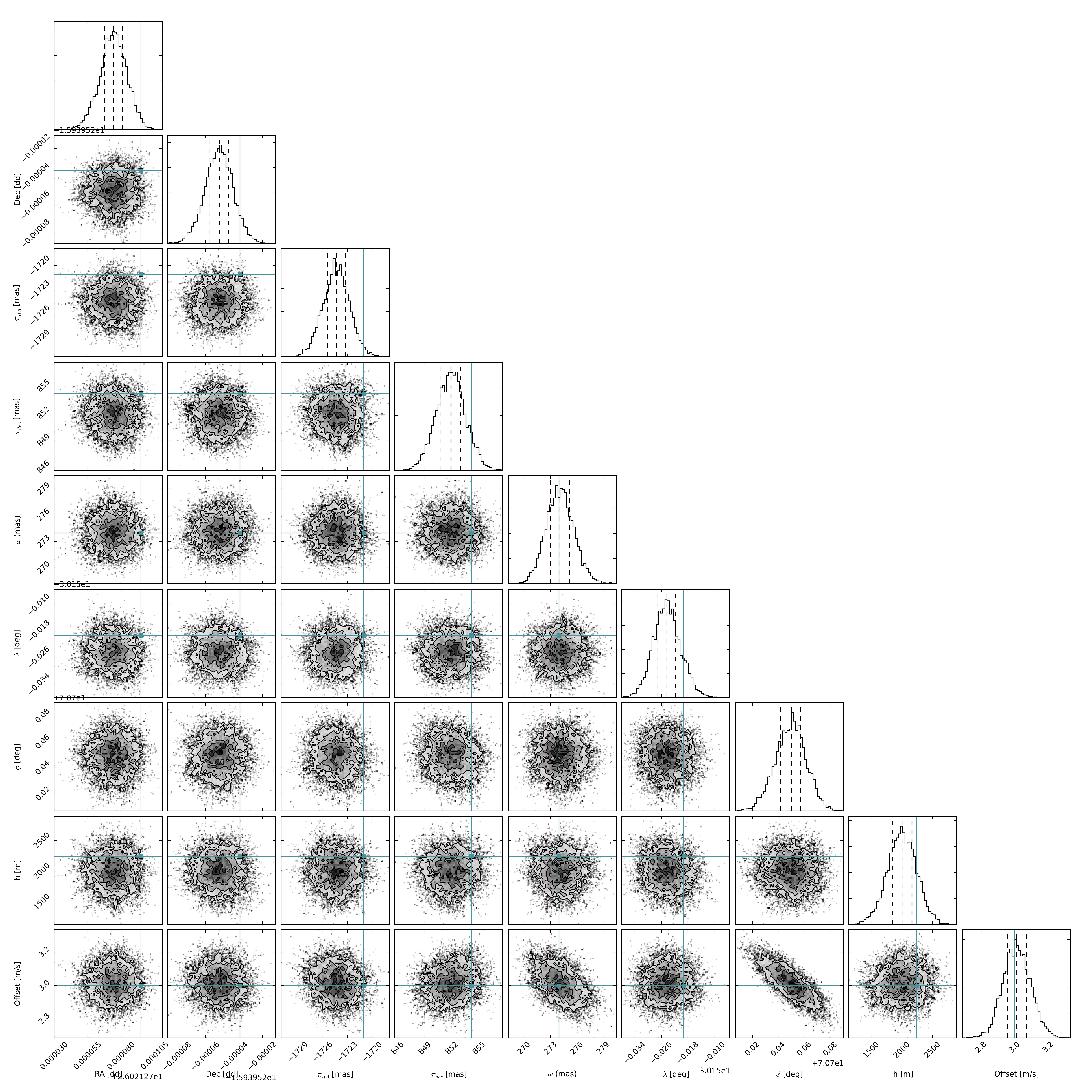
I then said the burn-in period completed in about 200 steps, cut those out, and below are the resulting distributions from sampling the posterior.
The median values for each parameter were then fed into barycorr. This reduced the RMS, but
still not below the value from the old barycorr.
| Method | RMS |
|---|---|
| Old Barycode | 2.178 m/s |
| Barycorr J2000- Hip & Mam vals | 2.722 m/s |
| Barycorr /hip - Hip & Mam vals | 2.474 m/s |
| Barycorr /hip - MCMC vals | 2.467 m/s |
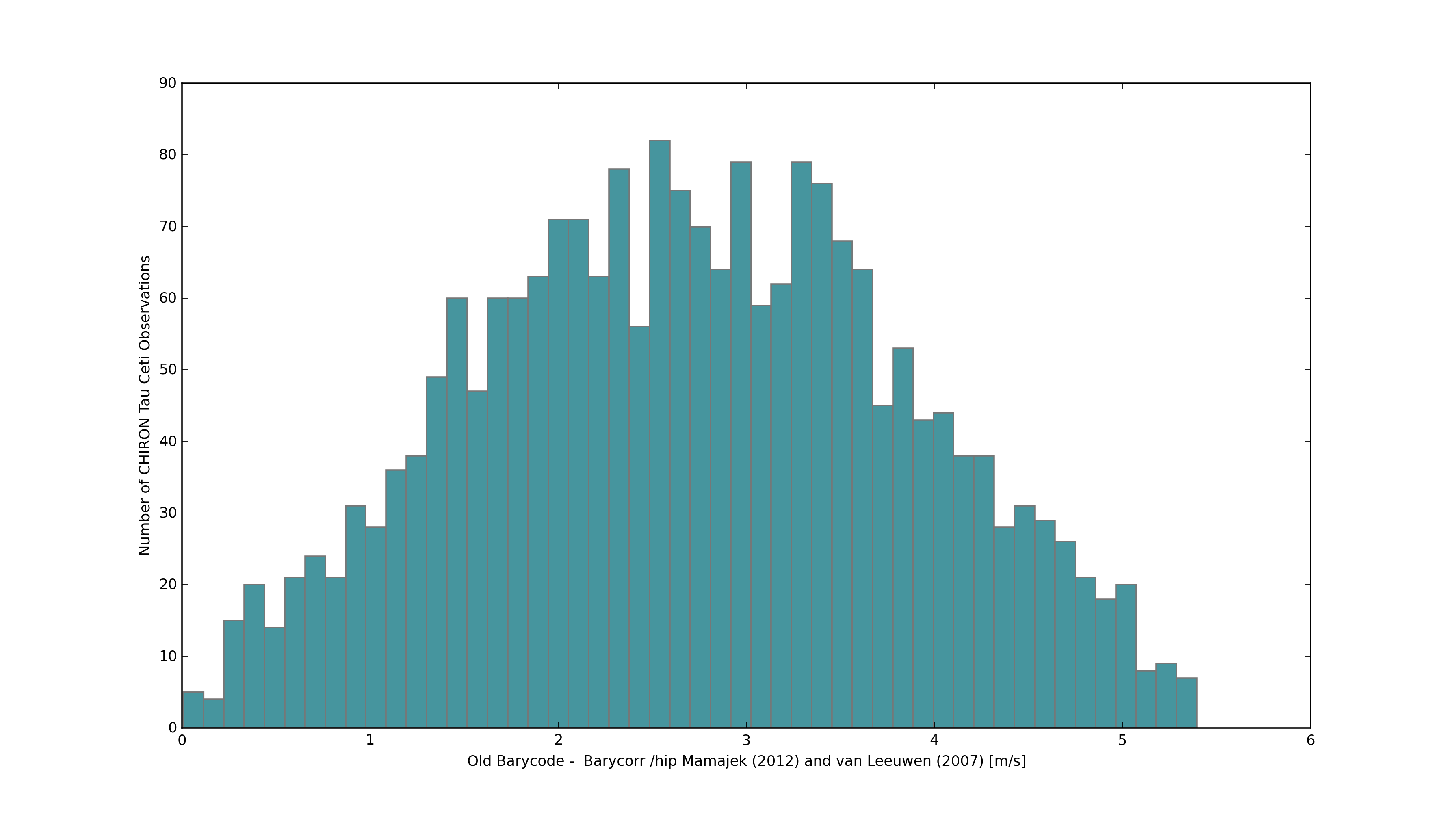
I then looked into whether or not any structure existed between the old barycentric correction and the new. The time series of the (“Old Barycode” - “Barycorr with Mamajek (2012) and van Leeuwen (2007) (1991.25 Epoch)) residuals is shown below.
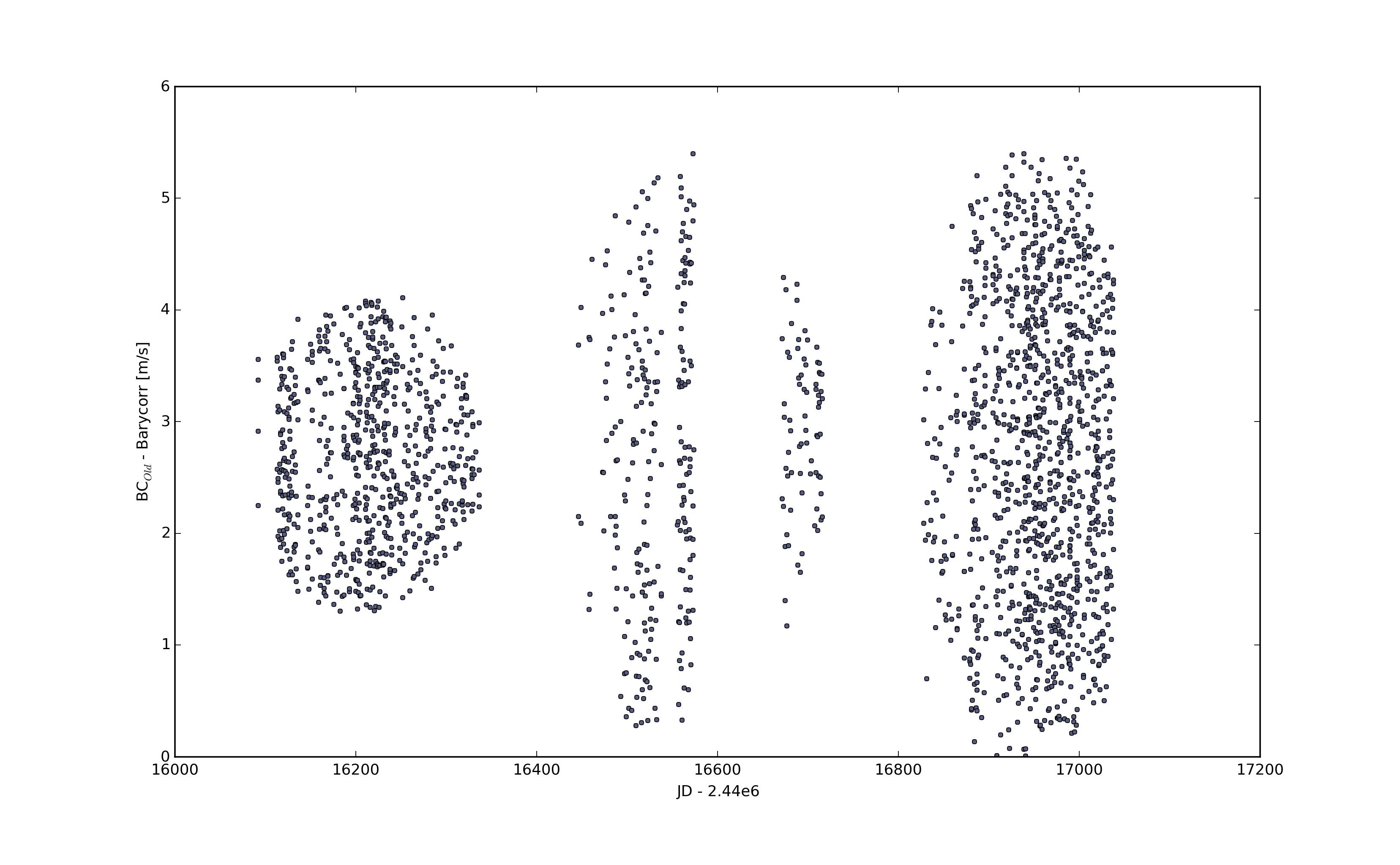
I was a little surprised to see the lack of structure in the residuals. I was expecting something with maybe an annual, semi-annual, or at least periodic signal. Looking at the distribution of the residuals shows nothing strange — they appear roughly normally distributed about some offset. Since we’re only concerned with differential RVs, the offset isn’t a big deal. I know we’ve seen this before.
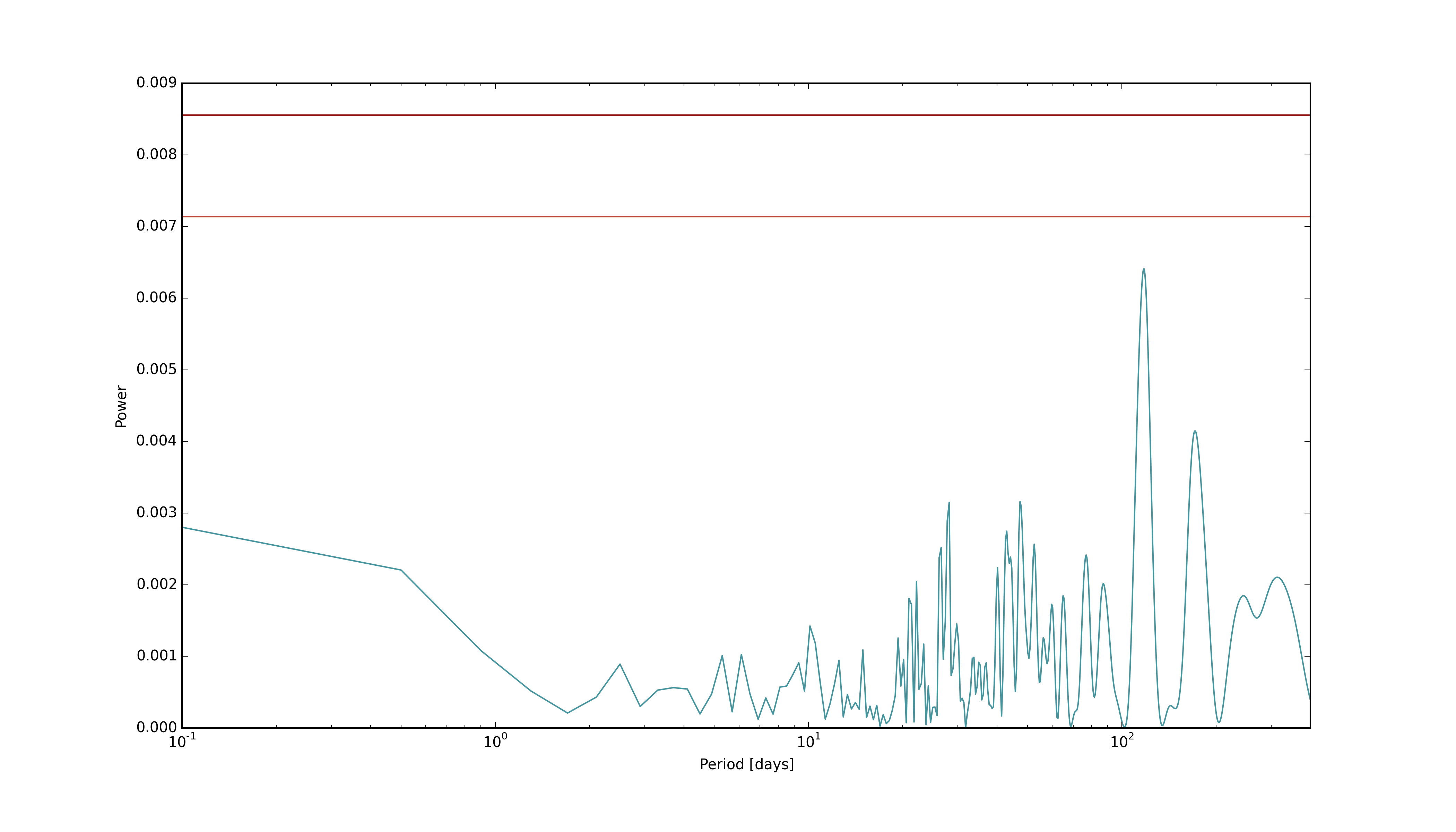
And looking at a periodogram of the time series shows nothing significant. Below is a plot showing the periodogoram of the same data set: Old barycode - Barycorr with Mamajek (2012) CTIO 1.5 m, van Leeuwen (2007), and 1991.25 Epoch. The superimposed horizontal lines are the 95% and 99% confidence levels based on a Boostrap MC analysis. These show that there is no significant power at any period between 0.1 and 400 days. The highest peak is at a period of 117.79 days, and the second highest peak is at period of 171.43 days.